Home

Battling the Non-Stationarity in Time Series Forecasting via Test-Time Adaptation

Jaebyeong Jeon / November 2025 (849 Words, 5 Minutes)

Abstract

Deep Neural Networks have spearheaded remarkable advancements in time series forecasting (TSF), one of the major tasks in time series modeling. Nonetheless, the non-stationarity of time series undermines the reliability of pre-trained source time series forecasters in mission-critical deployment settings. In this study, we introduce a pioneering test-time adaptation framework tailored for TSF (TSF-TTA). TAFAS, the proposed approach to TSF-TTA, flexibly adapts source forecasters to continuously shifting test distributions while preserving the core semantic information learned during pre-training. The novel utilization of partially-observed ground truth and gated calibration module enables proactive, robust, and model-agnostic adaptation of source forecasters. Experiments on diverse benchmark datasets and cutting-edge architectures demonstrate the efficacy and generality of TAFAS, especially in long-term forecasting scenarios that suffer from significant distribution shifts.

Motivation

• Time series data in real-world have non-stationary property → distributional discrepancy is increasing during test-time

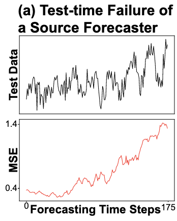
• Pre-trained forecaster becomes unreliable → need to adapt continuously during test-time while maintaining the prior core semantic (the idea of Test-Time Adaptation)

Task Definition & Formulations

• TSF: Predicting the future horizon window of H time steps (${x_{t+1}, … , x_{t+H}}$) given the past look-back window of L time steps (${x_{t-L+1}, … , x_t}$)
• $x_t \in \mathbb R^C$ denotes C number of variables observed at time t
• Time series forecaster $\mathcal F_\theta: \mathbb R^{L\times C} \rightarrow \mathbb R^{H \times C}$
• $(X_t, Y_t) = ({x_{t-L+1}, …, x_t}, {x_{t+1}, … ,x_{t+H}})$

Differences with TTA in Computer Vision

• Access to test labels is available
  • In real-world, it is not available to annotate the image during test-time → Assume complete absence of test labels
  • However, in time series data, the ground-truth labels become gradually accessible after each prediction step e.g., When forecasting electricity consumption for the next 30 days, the full ground-truth labels become available only after the entire 30-day period has passed
  • Before having access to the full set of ground-truth labels, a portion of them can still be observed e.g., In this case, the true consumption for the first 7 days becomes observable after one week, even though the remaining labels are not yet available → Use partially observed ground-truth labels for intermediate evaluation and adaptation
• The IID assumption does not hold
  • Time series data inherently exhibit autoregressive correlations → Addressing non-IIDness at both the local and global levels becomes an essential challenge in this setting

Overview of TAFAS

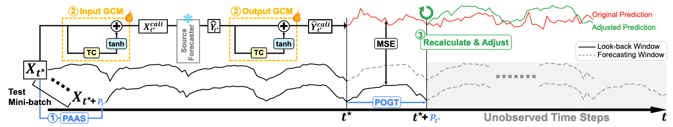
• Periodicity-aware adaptation scheduling (PAAS)
• Obtain partially-observed ground truth of sufficient length to represent semantically meaningful periodic patterns
• Gated calibration module (GCM)
• GCMs are adapted to calibrate test-time inputs such that they conform to the distribution the source forecaster effectively handles
• The gating mechanism in GCMs controls how much the calibrated results should be utilized by considering global distribution shifts
• Throughout the adaptation, the source forecaster remains frozen to preserve the core semantics it has learned from the extensive historical data
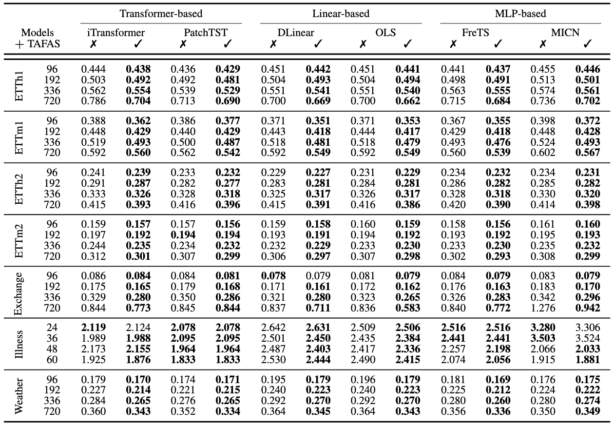
• TAFAS adjusts the latter part of the original predictions, where ground truths are yet to be observed, with the adapted predictions reflecting the distribution shift
• Large gain in long-term forecasting scenario which has prominent distribution shift
• The benefits become more pronounced in long-term forecasting scenarios where distribution shifts are more significant

PAAS

• PAAS extracts meaningful periodic patterns from the look-back window to determine the length of POGT
• Finding highest signal power by applying FFT and determine the dominant frequency based on the highest signal power:
  • $c^* = \underset{c} {\text{argmax}}\underset{f} {\sum}|\text{FFT}(X^c_{t_0})|^2$
  • $f^* = \underset{f}{\text{argmax}}|\text{FFT}(X^{c^*}_{t_0})|^2$
• The look-back window p is determined in the following manner:
  • $p_{t_0}=\big\lceil \frac {L}{f^*} \big\rceil$
• Once $p_{t_0}$ is determined, $p_{t_0}+1$ instances are aggregated into a test-mini-batch: \(\{X\}^{t_0 + p_{t_0}}_{t_0} = \{X_{t_0}, ..., X_{t_0 + p_{t_0}}\}\)
• When the subsequent look-back window arrives at time step $t_0 + p_{t_0}+1$, PAAS is repeated to calculate the subsequent length of POGT adaptively

GCM

• Input GCM maps the distribution-shifted test input to a calibrated input that belong in a distribution the source forecaster can handle
• Output GCM remaps the source forecaster’s prediction in order to calibrate the result back to the continuously changing test distribution
• Temporal calibration → linear transform / Global calibration → tanh gating mechanism
• $\text{GCM}(X_t)= X_t +\text{Tile}\big(\text{tanh}(\alpha)\big) \circ \big(\text{Concat}({W^cX^c_t}_{c=1}^C)+b \big)$
• GMC module update
  • $t^*$ denotes a time step at which PAAS calculates the POGT length ($t_0, t_0+p_{t_0}+1, …$)
  • \(p_{t^*}\) denotes the POGT computed at $t^*$
  • After a test mini-bath \(\{X\}_{t^*}^{t^*+p_{t^*}}\) is obtained at \(t^*+p_{t^*}\), GCMs are adapted by minimizing the TAFAS loss defined as the following:
    • \[\mathcal L^\text{partial}=\text{MSE}\big(\hat{Y}^\text{cali}_{t^*}\big [:p_{t^*}\big], Y_{t^*} \big [:p_{t^*} \big ] \big )\]
    • $\mathcal L^\text{partial}$ is computed between the first \(p_{t^*}\) time steps of the calibrated prediction for \(X_{t^*}\) whose periodicity-aware POGT is available (\(\hat{Y}^\text{cali}_{t^*}\big [:p_{t^*}\big]\)) and the corresponding POGT (\(Y_{t^*} \big [:p_{t^*} \big ]\))
    • \[\mathcal L^\text{full}=\text{MSE}\big(\{\hat{Y}^\text{cali}\}_{\tilde{t}^*}^{\tilde{t}^*+\tilde{p}_{\tilde{t}^*}}, \{Y\}_{\tilde{t}^*}^{\tilde{t}^*+\tilde{p}_{\tilde{t}^*}} \big )\]
    • $\mathcal L^\text{full}$ is calculated between the calibrated predictions of all look-back windows within the past mini-batch constructed at $\tilde {t}^* + p_{\tilde{t}^*}$ and the associated full ground truths
    • $\tilde{t}^*$ represents the most recent time step among the past POGT-computing steps whose corresponding mini-batches have now observed their full ground truths
    • $\mathcal L^\text{TAFAS} = \mathcal L ^\text{partial} + \mathcal L^\text{full}$

Prediction Adjustment (PA)

• TAFAS can replace the latter part of original predictions, whose ground truths are yet to be observed, with adjusted predictions that reflect the distribution shift
• After the forecaster is adapted at \(t^*+p_{t^*}\), TAFAS recalculates the predictions for all look-back windows in \(\{X\}_{t^*}^{t^*+p_{t^*}}\) and then substitues the original predictions for time steps after \(t^*+p_{t^*}\) with the adapted predictions
• For the look-back window \(X_{t^*+k}\), where \(k\in \{0,..., p_{t^*}\}\), the corresponding prediction \(\hat {Y}^\text{cali}_{t^*+k}\) predicts time steps \(\{(t^*+k+1), ..., (t^*+k+H)\}\)
• For the time steps \(\{(t^*+p_{t^*}+1), ..., (t^*+k+H)\}\) which are yet to be observed, TAFAS substitutes the original prediction \(\hat {Y}^\text{cali}_{t^*+k}\) with the adapted prediction \(\hat {Y}^\text{cali, adapted}_{t^*+k}\) that reflects distribution shifts as the following:
  • \[\hat {Y}^\text{adjust}_{t^*+k, i} = \begin{cases}\hat{Y}^\text{cali}_{t^*+k, i} & \text{if } i \leq (t^*+p_{t^*}) \\ \hat{Y}^\text{cali, adapted}_{t^*+k, i} & \text{if } i \gt (t^*+p_{t^*}). \end{cases}\]

Experiments